Reduction
Two methods make a network smaller without losing what matters: simplify removes the nodes that only continue a road, and connecting_subnetwork keeps only the roads that join a set of points. ConnectionPlanner turns the second into a plan for connecting schools to existing fibre.
Simplifying a network
OpenStreetMap draws a road as a chain of many short segments, so an unsimplified road network has a node at every bend. simplify removes the nodes that only continue a road and joins the edges on either side, the way osmnx's simplify_graph does. Networks from OSMRoadsHandler and OSMRoadsFetcher are simplified by default; simplify=False gives the raw network.
raw_kigali = handler.load_data(kigali, simplify=False)
started = time.perf_counter()
simple_kigali = raw_kigali.simplify()
print(raw_kigali)
print(simple_kigali, f"{time.perf_counter() - started:.2f} s")
SpatialNetwork(nodes=166,206, edges=342,706, directed=True, weight='length')
SpatialNetwork(nodes=23,722, edges=61,611, directed=True, weight='length') 0.36 s
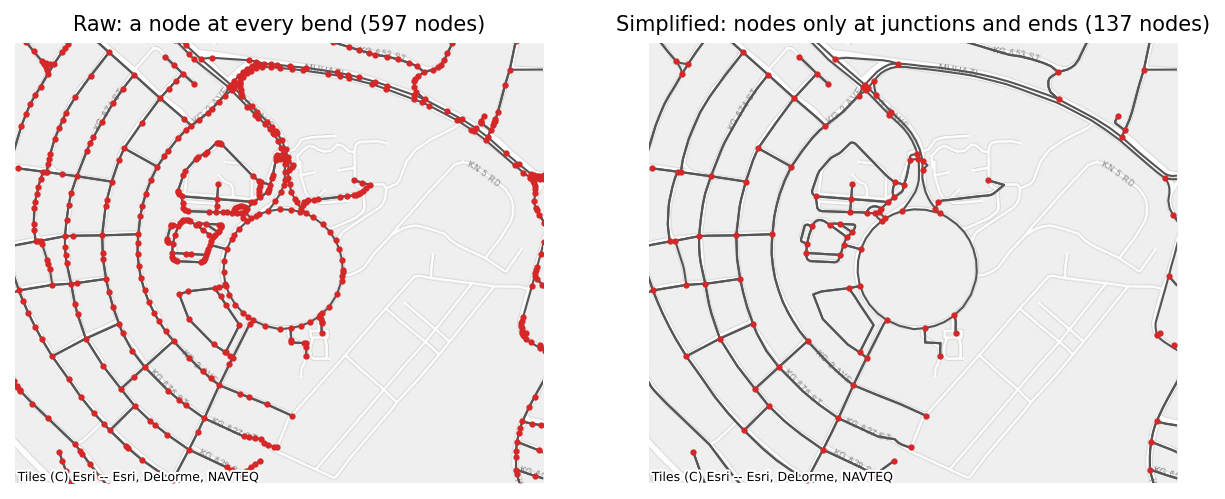
Which nodes go. A node is removed when it has exactly two neighbours and its edges continue through it: one edge in and one out of a one-way road, or both directions of a two-way road. In an undirected network, it is a node with exactly two edges. Nodes of kind point and split, and nodes passed in keep=, are never removed, so a network with inserted schools keeps its schools.
How joined edges are made. A joined edge's attributes come from the edges it replaces:
| Attribute | Rule |
|---|---|
length, the weight column, and columns in sum_columns | added up |
geometry | one line along the joined edges |
text, such as highway and name | joined with ; where the parts differ, without repeats |
osmid and other lists | concatenated, without repeats |
oneway | true only if every part is one-way |
reversed | true if any part is |
| other numbers | the length-weighted mean |
kind | the kind of the longest part |
joined = simple_kigali.edges[simple_kigali.edges["highway"].astype(str).str.contains(";")].iloc[0]
print(joined[["u", "v", "length", "osmid", "highway", "oneway"]])
u                        1224173076
v                        6370565775
length                   384.393696
osmid        [106060663, 680376414]
highway    unclassified;residential
oneway                        False
Name: 17137, dtype: object
Each direction of a two-way road is joined separately, so it stays two-way when both directions can be joined.
How it works. simplify never walks a chain of edges in Python. Each edge into a removable node is linked to the edge that continues it, which turns every chain into a linked list; pointer jumping ranks each edge's place in its chain in a logarithmic number of vectorised steps; and numpy's reduceat aggregates the attributes of every chain at once. On Rwanda's unsimplified network of 4.5 million edges this takes 7 s, against 148 s for osmnx, with the same nodes and edge lengths.
Where it differs from osmnx. osmnx also removes the nodes between two duplicated parallel ways and drops one of the ways, and it deletes rings that have no junction at all, such as a roundabout mapped on its own. simplify keeps both, so no road is lost. Neither occurs often; in Rwanda's roads, neither occurs at all.
Keeping the roads that connect a set of points
connecting_subnetwork answers a fibre planner's two questions: which roads would join these schools to each other, and which roads would connect them to the fibre that already exists, at the smallest total length? It keeps the part of the network that does it, and contracts it to the points, the fibre nodes, and the places where the paths branch. It works on the undirected network, since a cable laid along a road ignores one-way restrictions. Behind it is ConnectionPlanner (see Connection plans below), which also says how each school is connected and how far the plan can be from the best one.
inserted = set(network.node_index)
school_ids = [school for school in schools["school_id"] if school in inserted]
fibre_ids = [fibre for fibre in fibre_nodes["fibre_id"] if fibre in inserted]
clinic_ids = [clinic for clinic in clinics["clinic_id"] if clinic in inserted]

for label, call in [
    ("one tree joining the schools", lambda: network.connecting_subnetwork(school_ids)),
    ("the schools connected to the fibre", lambda: network.connecting_subnetwork(school_ids, roots=fibre_ids)),
    ("each school to its nearest fibre node", lambda: network.connecting_subnetwork(school_ids, roots=fibre_ids, method="nearest_root")),
    ("all pairs, 30 schools and the fibre nodes", lambda: network.connecting_subnetwork(school_ids[:30], roots=fibre_ids, method="all_pairs")),
]:
    started = time.perf_counter()
    result = call()
    print(f"{label}: {result.total_length() / 1000:.1f} km, {len(result.edges)} edges, {time.perf_counter() - started:.2f} s")
one tree joining the schools: 254.7 km, 501 edges, 2.70 s
the schools connected to the fibre: 249.7 km, 497 edges, 1.71 s
each school to its nearest fibre node: 355.2 km, 526 edges, 0.07 s
all pairs, 30 schools and the fibre nodes: 424.7 km, 748 edges, 0.84 s
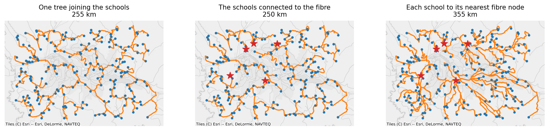
Open the interactive version of this map to zoom in on the routes.
Terminals and roots. The points to connect are the terminals. Roots, passed as roots=, are nodes already connected to each other through an existing network, such as fibre nodes, so reaching any of them is enough. Without roots, the result joins the terminals to each other.
The Steiner tree. The shortest set of roads that joins all the terminals is a Steiner tree, which may use road junctions as branching points. Finding it is NP-hard, so the library offers two approximations, each never more than twice as long as the shortest possible tree, \(2(1 - 1/\ell)\) times it for \(\ell\) leaves, and in practice within a few percent:
method="shortest_path"(the default) is Takahashi and Matsuyama's: start from the roots, or from the first terminal, and repeatedly connect the terminal nearest to anything connected so far, along its shortest path. After each connection, a Dijkstra from the new path updates every node's distance to the connected set, and stops wherever a distance does not fall, so it only searches the area the new path wins. 1.1 s for 1,000 schools on Rwanda's roads.method="steiner"is Mehlhorn's, 5 to 20 times faster and a few percent longer:- One multi-source Dijkstra from all the points gives every node its nearest point, which splits the network into one region per point (a Voronoi partition by road distance).
- Every edge whose ends lie in two different regions is a candidate link between those two points, with a length of the distance from each end to its point plus the edge itself. The cheapest link is kept for each pair of points.
- A minimum spanning tree over those links picks the pairs to join. Each chosen link is expanded back into its road path.
- A second minimum spanning tree over the roads in those paths removes any cycles, and leaves that are not points are pruned.
With roots, one virtual root. Joining every root to one extra node, a virtual root, at length 0 turns "connect every school to some fibre node" into a Steiner tree over the schools and that virtual root, which both methods solve as they are. Removing the virtual root leaves a forest whose every tree reaches a fibre node, so a school may connect through another school, and a road shared by several schools counts once. That is why the plan to the fibre above is much shorter than each school's own path to its nearest fibre node.
method="nearest_root". Each point takes its shortest path to its nearest root, and the result is the union of those paths. Schools share a road only where their own shortest paths overlap. One multi-source Dijkstra from the roots gives every point its nearest root and the path to it.
method="all_pairs". The shortest path between every point and every other point or root, as Giga's earlier code computed it. It shows every route that might matter, but the number of paths grows with the square of the number of points, so keep it for small sets.
In every case, the paths are collected from Dijkstra's predecessor arrays all at once, and the result is contracted with simplify(keep=points and roots), so it keeps the points, the roots, and the branching nodes, with lengths added up and geometries joined. weight="cost" minimises another column, such as the cost of laying fibre (see Worked use cases). A point that cannot be connected stays in the result as a node without edges.
Connection plans
ConnectionPlanner makes the same plans, and returns a ConnectionPlan: the contracted network, the chosen road edges as they are in the network, the cost, and a table with one row per school.
from gigaspatial import ConnectionPlanner

planner = ConnectionPlanner(network, school_ids, roots=fibre_ids)
plan = planner.plan()
print(plan)
print(plan.terminals.head())
ConnectionPlan(method='shortest_path', cost=249,675.9, terminals=197 of 197 connected, edges=1,970)
               status       root      distance  bridged  order  marginal_cost
node_id
school-000  connected  fibre-002  11592.441273    False     42     952.009015
school-001  connected  fibre-002   5065.420040    False     78    1091.600048
school-002  connected  fibre-002   3177.332951    False     21    1728.637288
school-003  connected  fibre-000   9581.415906    False    103    1530.212553
school-004  connected  fibre-000   3400.977858    False     18    1404.324554
status is connected, root for a school that is itself a fibre node, or unreachable for one that no road joins to any root. root is the fibre node its part of the plan reaches nearest, and distance the length along the plan to it. order and marginal_cost come from shortest_path: when the school was connected, and the length its connection added. They make the plan a phased rollout (see Worked use cases).
Improving a plan, and how good it is. improve shortens a plan by local search and never makes it worse, and lower_bound computes a length that no plan can go below:
started = time.perf_counter()
better = planner.improve(plan)
bound = planner.lower_bound(better)
print(f"{plan.cost / 1000:.1f} km, improved to {better.cost / 1000:.1f} km in {time.perf_counter() - started:.1f} s")
print(f"No plan is shorter than {bound / 1000:.1f} km, so this one is at most {better.gap:.1%} above the best.")
249.7 km, improved to 244.1 km in 4.7 s
No plan is shorter than 241.0 km, so this one is at most 1.3% above the best.
improve repeats two moves until neither helps. Key-path exchange removes a stretch of the plan between two schools, fibre nodes, or branching junctions, and reconnects the two halves by the cheapest path between them. Key-vertex elimination removes a branching junction and its stretches, and reconnects the pieces by their cheapest links. Either is kept only when it saves length. lower_bound is Wong's dual ascent: on the network with both directions of every road, it grows the set of nodes that reach each school at no extra cost, raising the bound by the cheapest road into that set, always for the school whose set has the fewest roads into it, until every school's set reaches the fibre. time_limit= stops either early.
How close to the best. Against exact optima, from scipy's integer programming solver on Kigali's roads, and SteinLib's published optima for 78 standard random test graphs:
| Kigali's roads, 30 and 60 schools, 3 fibre nodes (10 instances) | SteinLib sets B to E (78 instances, mean) | |
|---|---|---|
steiner | 3.0 to 8.8% above the optimum | 3.4 to 9.9% above |
shortest_path | 0.65 to 5.9% above | 2.6 to 4.7% above |
either, then improve | 0.00 to 0.86% above | 0.4 to 2.2% above |
lower_bound | 0.07 to 1.1% below | 0.05 to 0.42% below |
On Rwanda's roads with 1,000 schools, improved plans have a gap of 1.4% to the bound. The design and algorithm decisions give the benchmarks.
Bridges. In a network with parts that no road joins, such as a clipped area or one loaded with retain_all=True, schools in a part without fibre are unreachable. bridge_cost= lets the plan use straight-line links between parts, such as microwave links, at a cost per metre and up to bridge_max_distance metres; a plan uses one only where it is cheaper than the roads:
# not run
planner = ConnectionPlanner(clipped, school_ids, roots=fibre_ids, bridge_cost=3.0, bridge_max_distance=2000)
plan = planner.plan()
links = plan.edges[plan.edges["kind"] == "bridge"]
print(plan.terminals["bridged"].sum(), "schools are connected through a bridge")
Use cases. Fibre backbone planning and extension from existing fibre (with roots), a phased rollout (order and marginal_cost), and estimating the trench length or cost of a plan, which is the plan's cost, or total_length() of its network.
How a source is cut from an extract
OSMRoadsHandler stores each extract's whole network, uncropped, and cuts it to a source when it loads. To give the same network OSMRoadsFetcher would, it replays the steps of osmnx's graph_from_polygon:
- Widen the area. The source becomes an area by the fetcher's rules (a country's boundary, a geometry as given, a frame's union, or points' hull, bounding box, or buffers), and the area is widened by 500 m, as osmnx widens what it downloads. The raw network's nodes in the widened area are kept; with
truncate_by_edge=True, so are the nodes just outside that share an edge with one inside. - Combine extracts. When a source needs several extracts, such as schools along a border, their raw networks are combined as if they were one file: a road that crosses between extracts is in both, and is kept once.
- Keep the largest connected part, and simplify, unless
retain_all=Truekeeps every part. - Cut to the area. The nodes in the area itself are kept, and the largest connected part again.
street_countis the count on the simplified widened network, as osmnx sets it.
Simplifying the widened network before cutting it decides what happens to a road that leaves the area: its simplified edge runs to the next real junction outside, so the edge's far end is outside the area and the edge is dropped. That is what osmnx does, and the handler does the same, so a cropped load equals the fetcher's network for the same area. A country whose extracts are its own file, or its regional files, is not cropped at all.